Methods and Materials
The file images were saved into a folder designated for the purpose of organization and ease of selection. DS9 was downloaded from its official website and launched; an image was chosen and opened within the program. It was necessary to adjust the color, scale, and contrast of each image in order to effectively visualize the various objects in the particular image. Each raw image file featured a main central quasar. Using the tool region editing capabilities in DS9, circular regions with radii of 25, 40, 80, and 200 kiloparsecs surrounding the main QSO were created as survey regions. Parsecs, along attached with varying prefixes, are a common measurement used in astronomy and a kiloparsec is approximately equivalent to 3,262 light years. With the regions created, every visible and significant object was highlighted and numbered with the box tool.
For each object various data were collected, including the object’s distance to the central quasar in arcseconds, and the object’s right ascension and declination (celestial coordinates) in hour minute second format. The apparent visual disturbance and apparent galaxy type of the object was also recorded. The objects’ distances were identified with the ruler tool in DS9, whereas the coordinates were obtained by hovering the cursor over the object and reading the output shown at the upper left hand corner of the DS9 widget. By adjusting the color, contrast, and scale of the image, the apparent physical disturbances and galaxy morphologies were able to be identified for most, if not all, of the objects within the established survey regions.
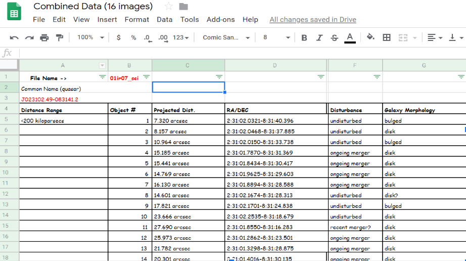
Figure 1 (above). One of the data tables created for organization in Google Sheets.
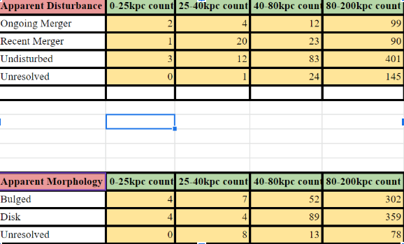
From the recorded data in Google Sheets, a collection of graphs were created to better visualize and establish correlations and patterns between the gathered information. The first graph was created by first making a table in Google Sheets with one section representing the apparent disturbances--ongoing [galactic] merger, recent merger, undisturbed, and unresolved--, and the other showing the 0 to 25 kiloparsec, 25 to 40 kiloparsec, 40-80 kiloparsec, and 80-200 kiloparsec regions and their object counts. The same was done for the second graph, except one section represented the apparent morphologies--bulged, disked, and unresolved appearances-- rather than disturbances, while the survey region section remained the same. The tables were filled with the proper object count in each box by looking at which regions each object resided in from DS9 and the first 16 data tables. These tables of information were then translated to graphical representations.
Figure 2 (below). A cropped screenshot of the two completed data tables created as the basis for the graphs.